Machine Learning
How Can We Help?
Get the most out of our software.
Machine Learning
THE AI/ML MODEL.
Once good data has been captured from the production recipes, this data is then broken up on a per sensor and per recipe basis. For each recipe a single machine learning model is trained per sensor. In many machine learning applications, a model is trained to classify between one of n classes. The goal is to determine when the component/equipment is behaving abnormally. Formally this is framed as an anomaly detection problem. Therefore, we will initially train a model to recognize what normal production looks like, and then over time, as anomalous states are encountered, incorporate them into the training datasets.
The first step in creating the model is feature extraction from the streaming raw sensor data. In this write-up, we refer to Bosch XDK’s (XDK), but, user can deploy any type of sensor. The Bosch XDK’s are capable of streaming numerous types of sensor data, and the readings that our models are trained with incorporate acceleration in the x,y, and z directions as well as angular acceleration in the x,y, and z directions. This means that for every sample in time, six readings are being ingested by the ML model. With most time series data, a single timestep is not necessarily useful, but rather a series of timesteps must be processed at once in order to make meaningful inference from the data. When training and running a model, this is accomplished via a sliding window, who’s step size and length is optimized as part of a hyperparameter search during training. A set of features are calculated based on all of the samples that fall within a window, and then the ML model can process the entire time series as a single set of higher level features.
While features can be manually fine-tuned, they can also be optimally found through the use of grid search or genetic algorithms, the latter being the techniques that we use when extracting features. Once the optimal features have been found, a model can be trained and built. Because the goal of the ML application is to identify anomalous behavior, we use a neuron based machine learning algorithm to learn bounds on clusters of data. A two dimensional rendering of what one of these neurons looks like is shown below. The bounding box is defined by an area of influence, and both the center, as well as this area of influence, are what is learned during training. As the model is exposed to more training data, it is able to learn more complicated clusters and structure by creating new neurons or modifying the center/area of influence of existing neurons.
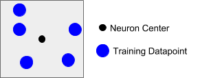
Figure 11: Neuron Example
The training datapoints are shown in blue, while the center of the neuron is shown in black and the bounding box signifies the area of influence of the neuron.
At runtime, the streaming samples are collected into windows of length l as tuned during training, and once enough samples have been captured to fill a window, features are calculated and the ML model is able to make a classification decision. It is assumed that any points falling within the bounds of an existing neuron are part of a known class, and any points falling outside of these bounds are part of an unknown, or anomalic class. How anomalies are detected and handled will be expanded on in the section below.